Merging data frames

When looking at the HIV, life expectancy, worldbank data and countries data frames, we saw that worldbank data is tidy, therefore we applied pivot_longer to both of the HIV prevalence and life expectancy data frames so that they can be compatible with the worldbank data frame. Furthermore, looking at the date ranges in all the data frames:

• hiv -> 1979 to 2011
• life_expectancy -> 1800 to 2064
• worldbank_data -> 1960 to 2016

We decided to attach HIV and life expectancy to worldbank_data using the left join function in order to preserve the optimal date range.

life_long <- life_expectancy %>% 
  pivot_longer(
    cols = 2:302,
    names_to = "date",
    values_to = "life_expectancy"
    ) %>% 
  mutate(date = as.numeric(date))

hiv_long <- hiv %>% 
  pivot_longer(
    cols = 2:34,
    names_to = "date",
    values_to = "HIV"
) %>% 
  mutate(date = as.numeric(date))

countries_tidy <- countries %>% 
  select(c(3,9))

worldbank_merge <- worldbank_data %>% 
  left_join(countries_tidy, by = c("country"))
            
            
worldbank_merge2 <- worldbank_merge %>% 
  left_join(hiv_long, by = c("country", "date")) %>% 
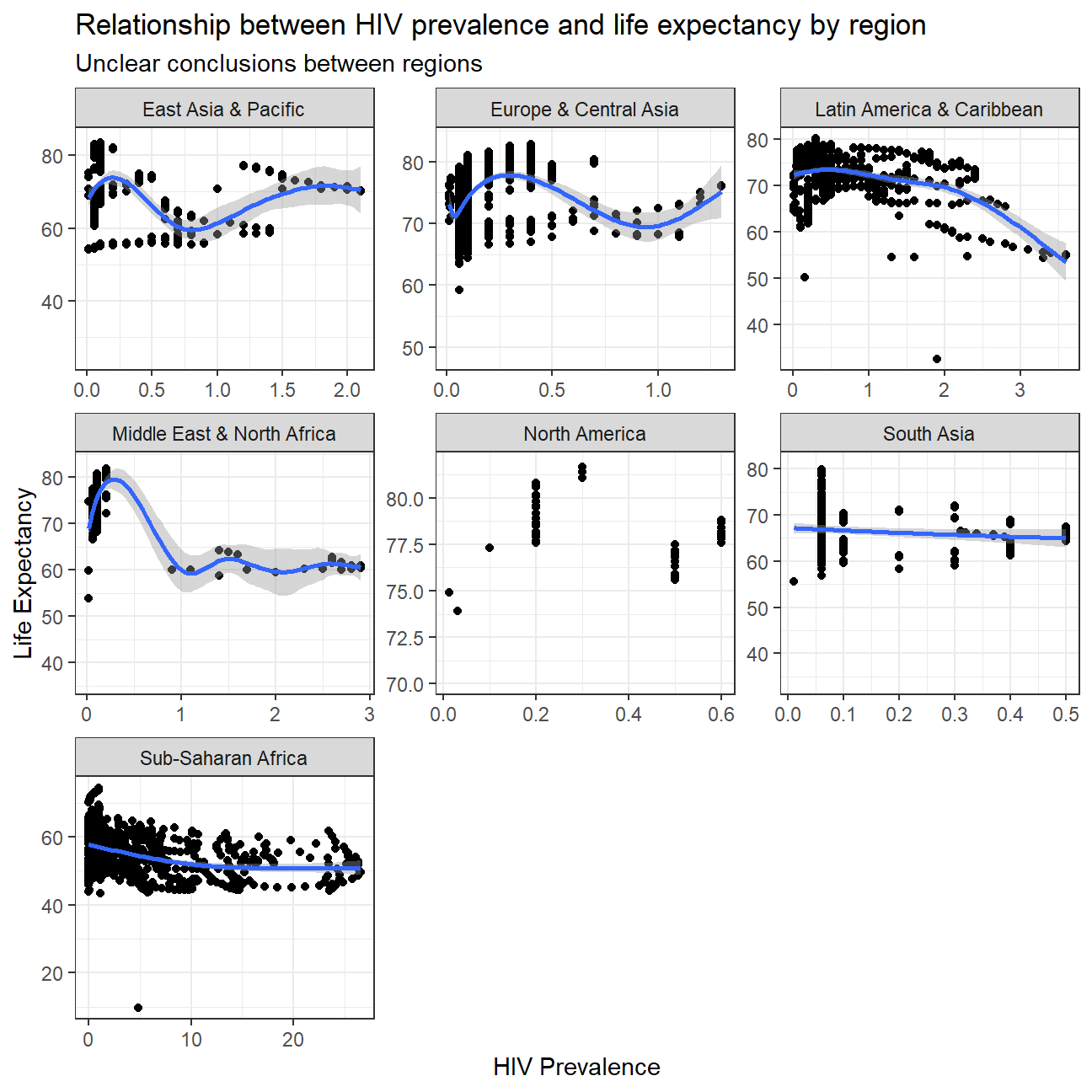
  left_join(life_long, by = c("country", "date")) 

Looking at the relationship between HIV prevalence and life expectancy

The graph below illustrates that particularly in the Middle East & North Africa, Latin America & Caribbean, Sub-Saharan Africa there is a clear relationship showing that with higher levels of HIV prevalence, life expectancy declines, this can be expected as, particularly in the past, the disease would virus was life threatening. However, East Asia & Pacific, and Europe & Central Asia show some ambiguous results. Perhaps showing the relationship between HIV prevalence and life expectancy is picking up the indirect effects of other factors such as poor health infrastructure or lower sanitary standards.

worldbank_merge2 %>% 
ggplot(mapping = aes(x=HIV, y=life_expectancy)) +
         geom_point() +
          geom_smooth() +
          facet_wrap(~region,scales = "free") +
          theme_bw() +
          labs(title = "Relationship between HIV prevalence and life expectancy by region",
            subtitle = "Unclear conclusions between regions",
              x = "HIV Prevalence",
               y = "Life Expectancy"
            )

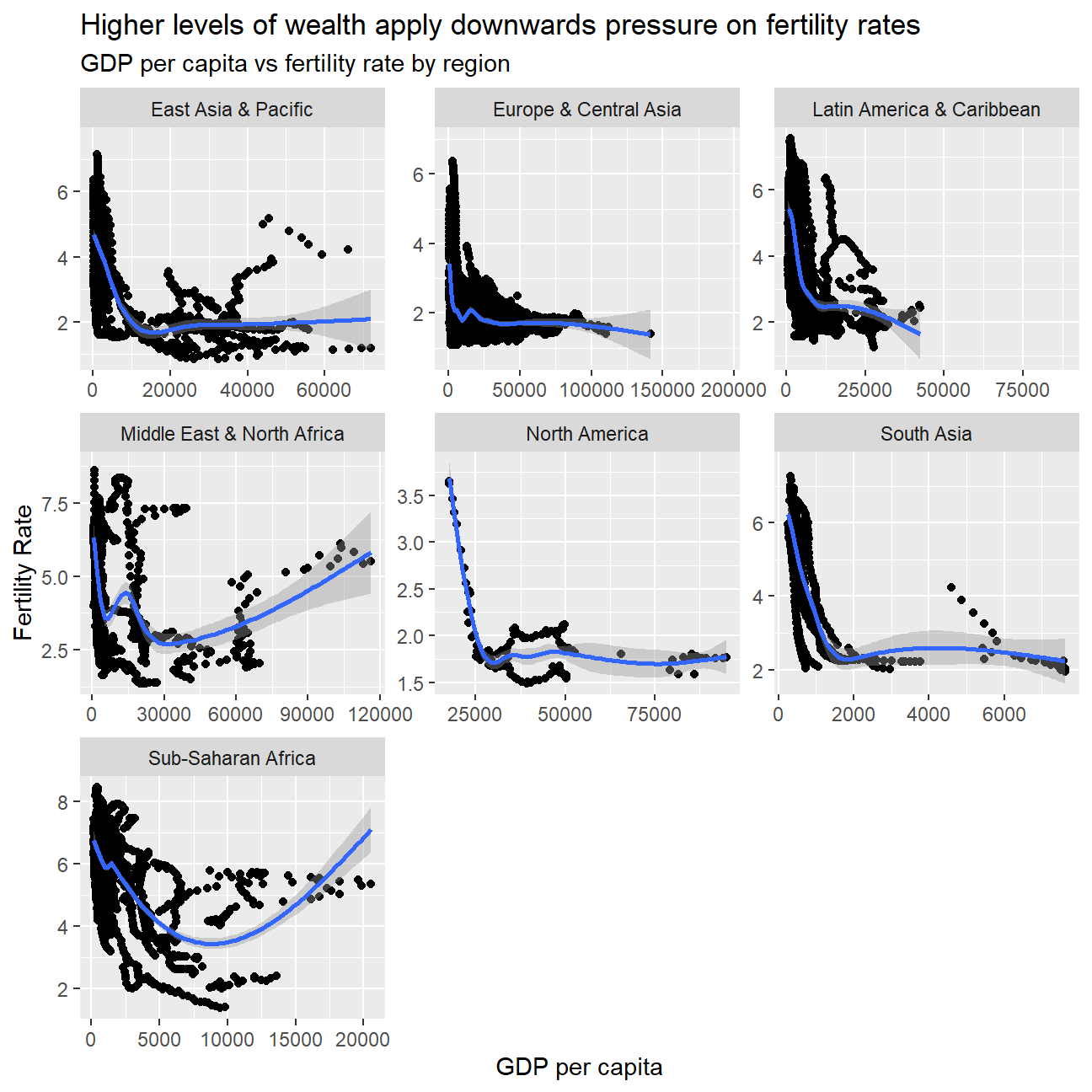
Examining the effects of GDP per capita on fertility rates

Higher levels of wealth, here measured by GDP per capita, are negatively correlated with fertility rates. This relationship likely comes about as a result of better health care, better education and higher economic participation of women that often coincide with GDP growth.

worldbank_merge2 %>% 
ggplot(mapping = aes(x=NY.GDP.PCAP.KD, y=SP.DYN.TFRT.IN)) +
         geom_point() +
          geom_smooth() +
          facet_wrap(~region, scales = "free") +
          labs(
            x = "GDP per capita",
            y = "Fertility Rate",
            title = "Higher levels of wealth apply downwards pressure on fertility rates ",
            subtitle = "GDP per capita vs fertility rate by region"
          )

Missing HIV data

The region with the most missing observations is Europe & Central Asia with 996 NA values in this data frame, however since there are varying amounts of countries between the regions it is relevant to look at these in terms of a proportion to the total amount of potential observations. When looking at it from that perspective the East Asia & Pacific region misses the highest proportion with 74.1% of potential observations in the dataset registering NA.

hiv_missing <- worldbank_merge2 %>%
  group_by(region) %>% 
  filter(date >= 1979) %>% #the date range for HIV observations
  filter(date<= 2011)  %>% 
  summarize(hivNA = sum(is.na(HIV)), proportion = round(hivNA/n(),digits=3)) %>% 
  arrange(desc(hivNA))

#Absolute values
ggplot(hiv_missing,aes(x=reorder(region,hivNA),y=hivNA)) + 
  geom_col(fill = "lightslateblue") + 
  coord_flip() +
  theme_bw() +
  labs( x="",
        y="HIV missing data",
        title="Europe & Central Asia has the most missing HIV observations",
        subtitle="Number of missing HIV prevalence observations per region"
      )  +
  geom_text(aes(label=hivNA), vjust=0.5,hjust=1.5,angle=0, color="white", size=4)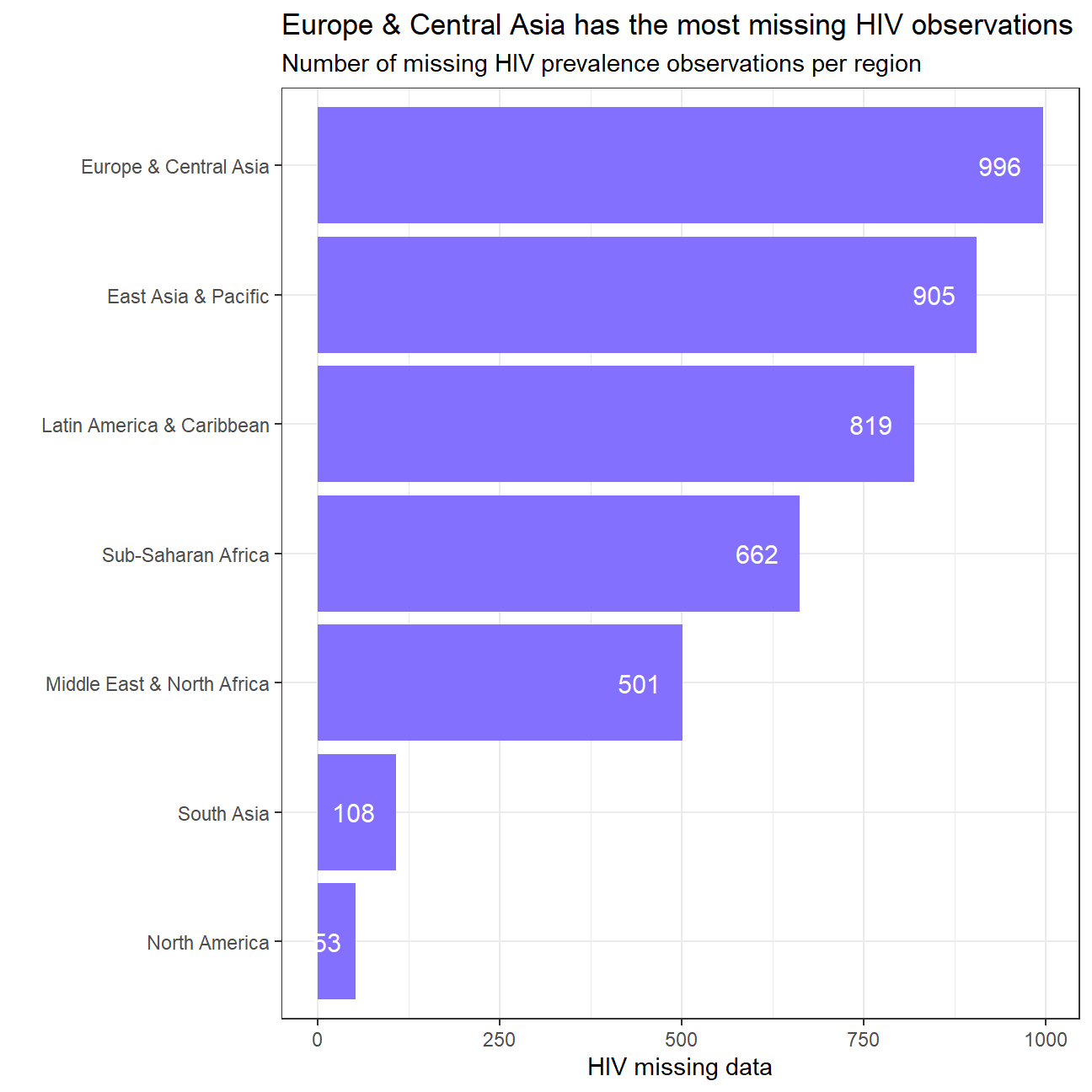

#Proportions
ggplot(hiv_missing,aes(x=reorder(region,proportion),y=proportion)) + 
  geom_col(fill="lightslateblue") + 
  coord_flip() +
  theme_bw() +
  labs( x="",
        y="HIV missing data",
        title="East Asia & Pacific has the most missing HIV data relative \nto the number of observations",
       subtitle="Proportion of missing HIV prevalence observations per region")  +
  geom_text(aes(label=scales::percent(proportion)), vjust=0.5,hjust=1.5,angle=0, color="white", size=4)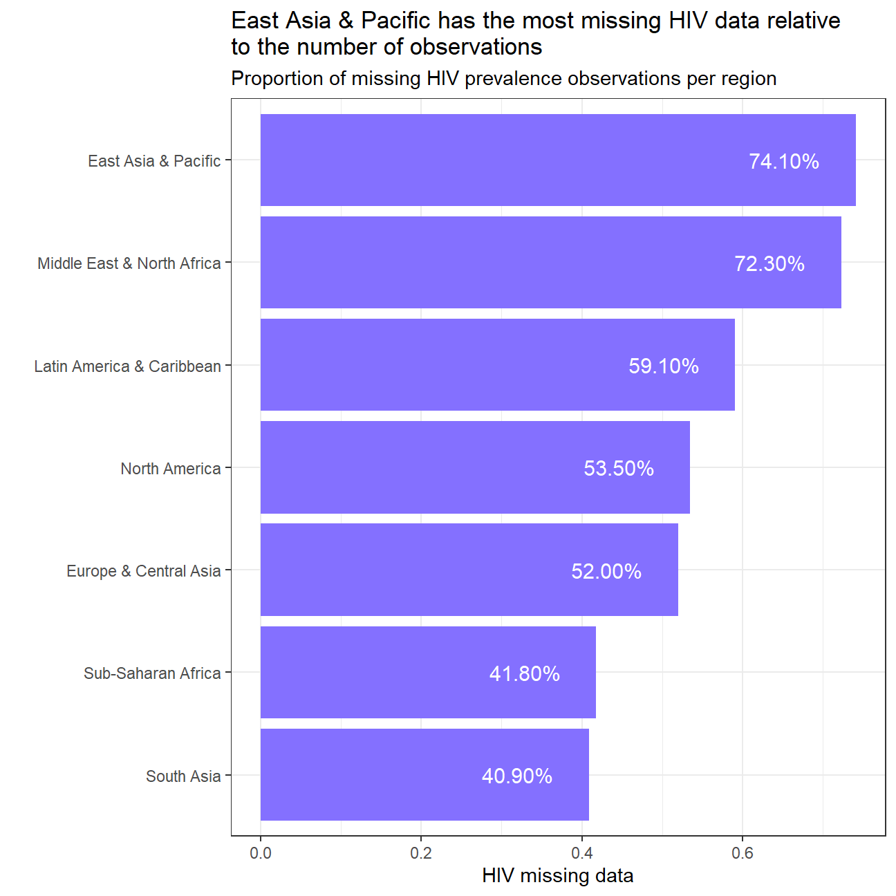 

Top 5 countries with the greatest/lowest decrease in mortality rate per region

When looking at the countries with the highest and lowest decreases in mortality, South Korea clearly comes out on time with a decrease of -96.97%, while globally Lesotho has had the slowest progress with their mortality rate dropping by only 51.525% over this time period. However, the conclusions you can draw from this analysis are pretty limited since some well developed countries such as Netherlands or the UK have experienced the slowest progress this is due to the fact that they were already well developed back in 1960. Another limitation of this analysis is the missing values of some countries that do not allow a comparison in the time period examined.

mortalityanalysis <- worldbank_merge2 %>%
                filter(date== "1960"| date=="2016") %>%
                select(c("country","region","date","SH.DYN.MORT")) %>% 
                pivot_wider(names_from="date", values_from="SH.DYN.MORT")
         
colnames(mortalityanalysis) = c("country","region","start","end")

mortalityanalysis_v2 <- mortalityanalysis %>% 
mutate(delta=(end-start)/start) %>% 
group_by(region) %>%
summarize(country,delta) %>%
arrange(region,desc(delta))

top_five <- mortalityanalysis_v2 %>%
            slice_min(order_by= delta,n=5) %>%
            summarize(country, delta)

ggplot(top_five,aes(x=reorder(country,desc(delta)),y=abs(delta))) +
  geom_col(fill="lightslateblue") + 
  coord_flip()+ 
  facet_wrap(~region,scales="free") + 
  labs(title="South Korea's monumental progress in mortality rate",
       subtitle="5 countries with the greatest decrease in mortality rate per region ",
       y="Change in mortality rate between 1960 and 2016",
       x="") +
  geom_text(aes(label=scales::percent(delta)), vjust=1,hjust=1, color="white", size=3)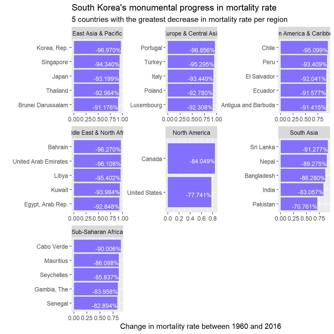 

bottom_five <- mortalityanalysis_v2 %>%
    slice_max(order_by= delta,n=5) %>%
  summarize(country,delta)


ggplot(bottom_five,aes(x=reorder(country,delta),y=abs(delta))) + 
  geom_col(fill="lightslateblue") + 
  coord_flip()+ 
  facet_wrap(~region,scales="free") + 
  labs(x="",
        y="Change in mortality rate between 1960 and 2016",
       title="Lesotho experienced the slowest progress in improving mortality worldwide",
       subtitle="Top 5 countries with the lowest decrease in mortality rate per region"
       ) +
  geom_text(aes(label=scales::percent(delta)), vjust=1,hjust=1, color="white", size=3)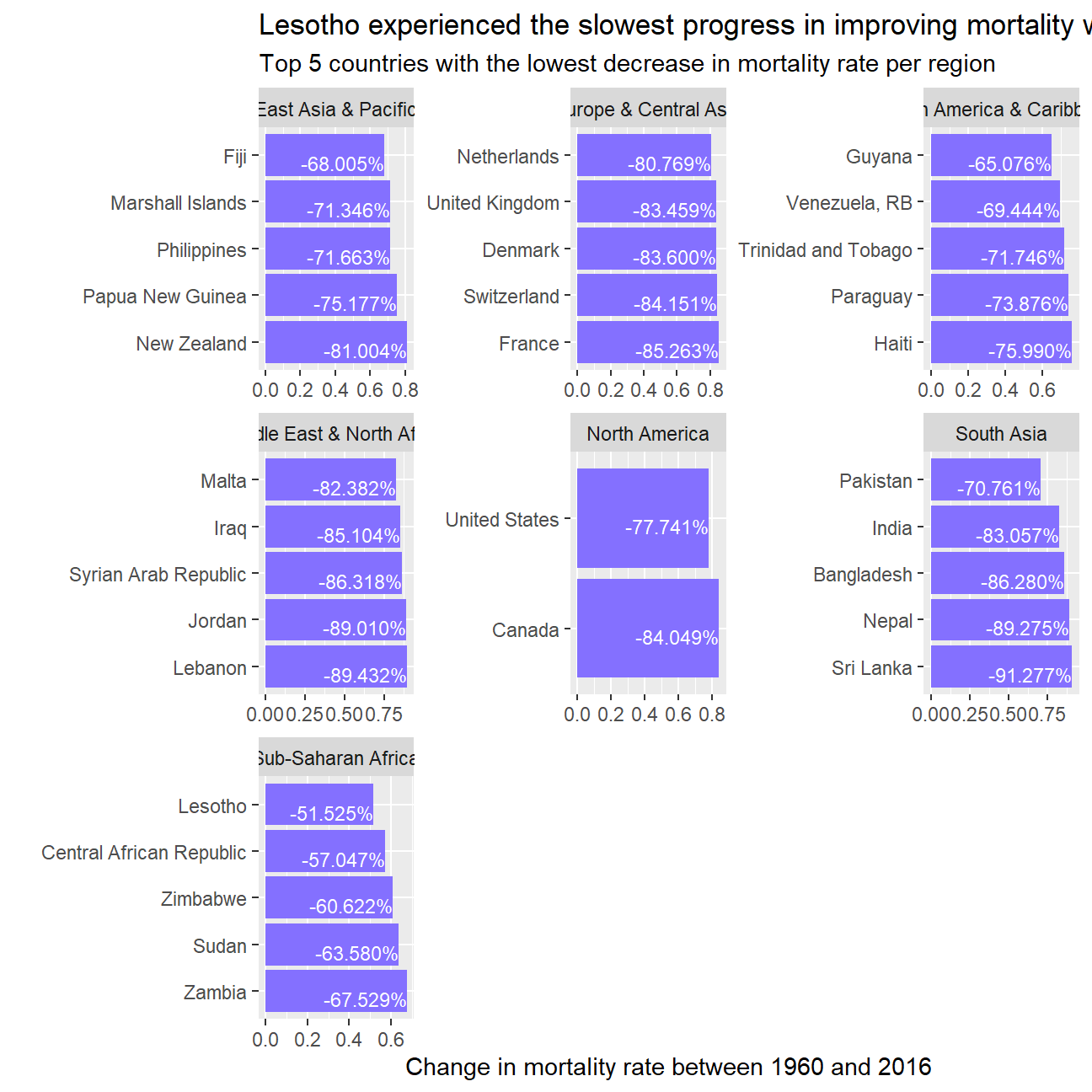 

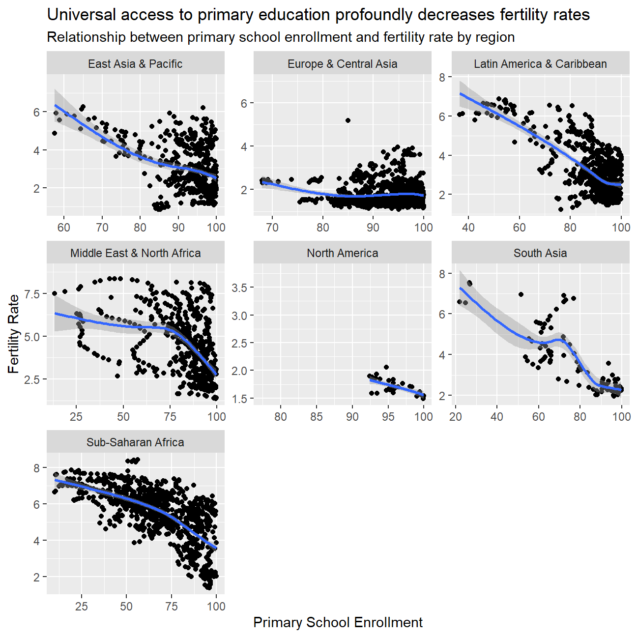
Is there a relationship between primary school enrollment and fertility rate?

There is a clear negative relationship between primary school enrollment and fertility rates. The higher proportion of the country that is able to obtain primary education the lower the fertility rate measures. Some may argue this illustrates a similar relationship as the previous relationship, however the correlation between education and fertility is even stronger, which underlines the role of education outcomes in this relationship. And the role of education has on health outcomes and on economic outcomes and independence of women.

worldbank_merge2 %>% 
ggplot(mapping = aes(x=SE.PRM.NENR, y=SP.DYN.TFRT.IN)) +
         geom_point() +
          geom_smooth() +
          facet_wrap(~region, scales= "free") +
          labs(x = "Primary School Enrollment",
               y = "Fertility Rate",
               title ="Universal access to primary education profoundly decreases fertility rates",
               subtitle = "Relationship between primary school enrollment and fertility rate by region"
               )