IMDB ratings: Differences between directors
Load the data and examine its structure
movies <- read_csv(here::here("data", "movies.csv"))
glimpse(movies)
## Rows: 2,961
## Columns: 11
## $ title <chr> "Avatar", "Titanic", "Jurassic World", "The Ave...
## $ genre <chr> "Action", "Drama", "Action", "Action", "Action"...
## $ director <chr> "James Cameron", "James Cameron", "Colin Trevor...
## $ year <dbl> 2009, 1997, 2015, 2012, 2008, 1999, 1977, 2015,...
## $ duration <dbl> 178, 194, 124, 173, 152, 136, 125, 141, 164, 93...
## $ gross <dbl> 7.61e+08, 6.59e+08, 6.52e+08, 6.23e+08, 5.33e+0...
## $ budget <dbl> 2.37e+08, 2.00e+08, 1.50e+08, 2.20e+08, 1.85e+0...
## $ cast_facebook_likes <dbl> 4834, 45223, 8458, 87697, 57802, 37723, 13485, ...
## $ votes <dbl> 886204, 793059, 418214, 995415, 1676169, 534658...
## $ reviews <dbl> 3777, 2843, 1934, 2425, 5312, 3917, 1752, 1752,...
## $ rating <dbl> 7.9, 7.7, 7.0, 8.1, 9.0, 6.5, 8.7, 7.5, 8.5, 7....# produce the data we will use today
Burton_Spielberg <- movies %>%
filter(director %in% c("Steven Spielberg", "Tim Burton"))Establishing the interval
g1 <- Burton_Spielberg %>%
  group_by(director) %>%
  summarize(n = n(),
            mean_rating = mean(rating, na.rm = TRUE),
            SD_directors = sd(rating, na.rm = TRUE),
            SE_directors = SD_directors/sqrt(n),
            t_critical = qt(0.975, n-1),
            lower95_ci = mean_rating - t_critical*SE_directors,
            upper95_ci = mean_rating + t_critical*SE_directors)

g1 %>%
  ggplot(mapping = aes(x = mean_rating, y= reorder(director, mean_rating)))+
  geom_point(aes(color = as.factor(director)), show.legend = FALSE, size = 5) +
  geom_errorbar(aes(xmin = lower95_ci, xmax = upper95_ci, color = as.factor(director)), width = 0.1, show.legend = FALSE, size = 1.8) +
  geom_rect(aes(xmin = max(lower95_ci), xmax = min(upper95_ci), ymin = -Inf, ymax = Inf), alpha = 0.1, fill = "black") +
  theme_minimal()+
  labs(x = "Mean IMDB Rating",
       y = "",
       title = "Do Spielberg and Burton have the same mean IMDB rating?",
       subtitle = "95% confidence intervals overlap"
       )+
  geom_text(aes(label = round(mean_rating,2)), vjust=-1, size=6)+
  geom_text(aes(x=upper95_ci, label = round(upper95_ci,2)), vjust=-1, size=5)+
  geom_text(aes(x=lower95_ci, label = round(lower95_ci,2)), vjust=-1, size=5)+
  NULL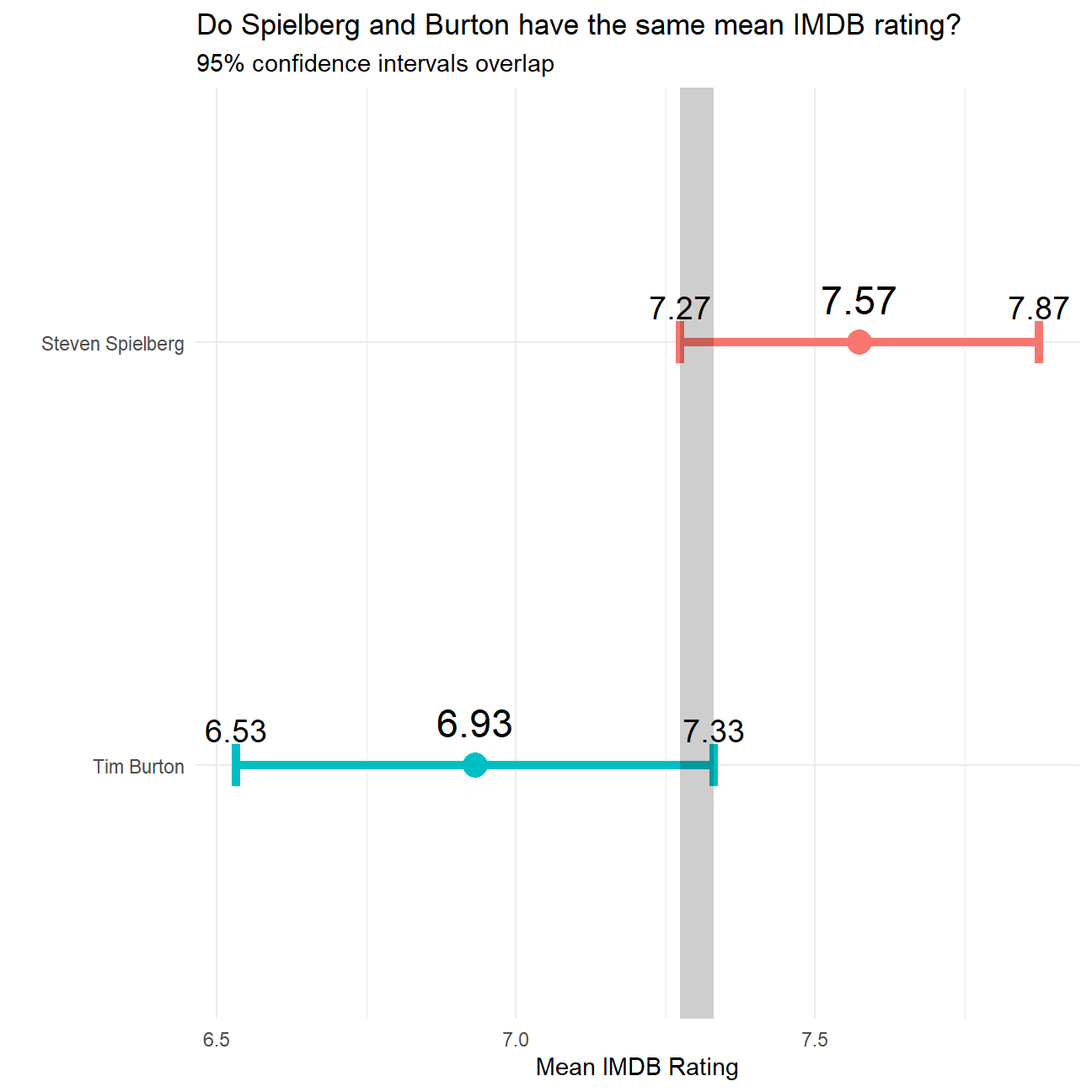
Hypothesis test with formula
- Null hypotheses: The mean IMDB rating for Steven Spielberg and Tim Burton are the same
- Alternative hypotheses: The mean IMDB rating for Steven Spielberg and Tim Burton are different
- p-value: if p-value is lower than 5%, then reject H0 and think the mean IMDB rating for Steven Spielberg and Tim Burton are different
t.test(rating ~ director, data = Burton_Spielberg)##
## Welch Two Sample t-test
##
## data: rating by director
## t = 3, df = 31, p-value = 0.01
## alternative hypothesis: true difference in means is not equal to 0
## 95 percent confidence interval:
## 0.16 1.13
## sample estimates:
## mean in group Steven Spielberg mean in group Tim Burton
## 7.57 6.93Hypothesis test with infer
- Null hypotheses: The mean IMDB rating for Steven Spielberg and Tim Burton are the same
- Alternative hypotheses: The mean IMDB rating for Steven Spielberg and Tim Burton are different
- p-value: if p-value is lower than 5%, then reject H0 and think the mean IMDB rating for Steven Spielberg and Tim Burton are different
# initialize the test, which we save as `directors_diff`
directors_diff <- Burton_Spielberg %>%
    specify(rating ~ director) %>%

    # the statistic we are searching for is the difference in means, with the order being "Steven Spielberg", "Tim Burton"
    calculate(stat = "diff in means", order = c("Steven Spielberg", "Tim Burton"))

# simulate the test on the null distribution, which we save as null
directors_null_dist <- Burton_Spielberg %>%
    specify(rating ~ director) %>%
    hypothesize(null = "independence") %>%
    generate(reps = 1000, type = "permute") %>%
    calculate(stat = "diff in means", order = c("Steven Spielberg", "Tim Burton"))

# Visualising to see how many of these null permutations have a difference
directors_null_dist %>% visualize() +
  shade_p_value(obs_stat = directors_diff, direction = "two-sided")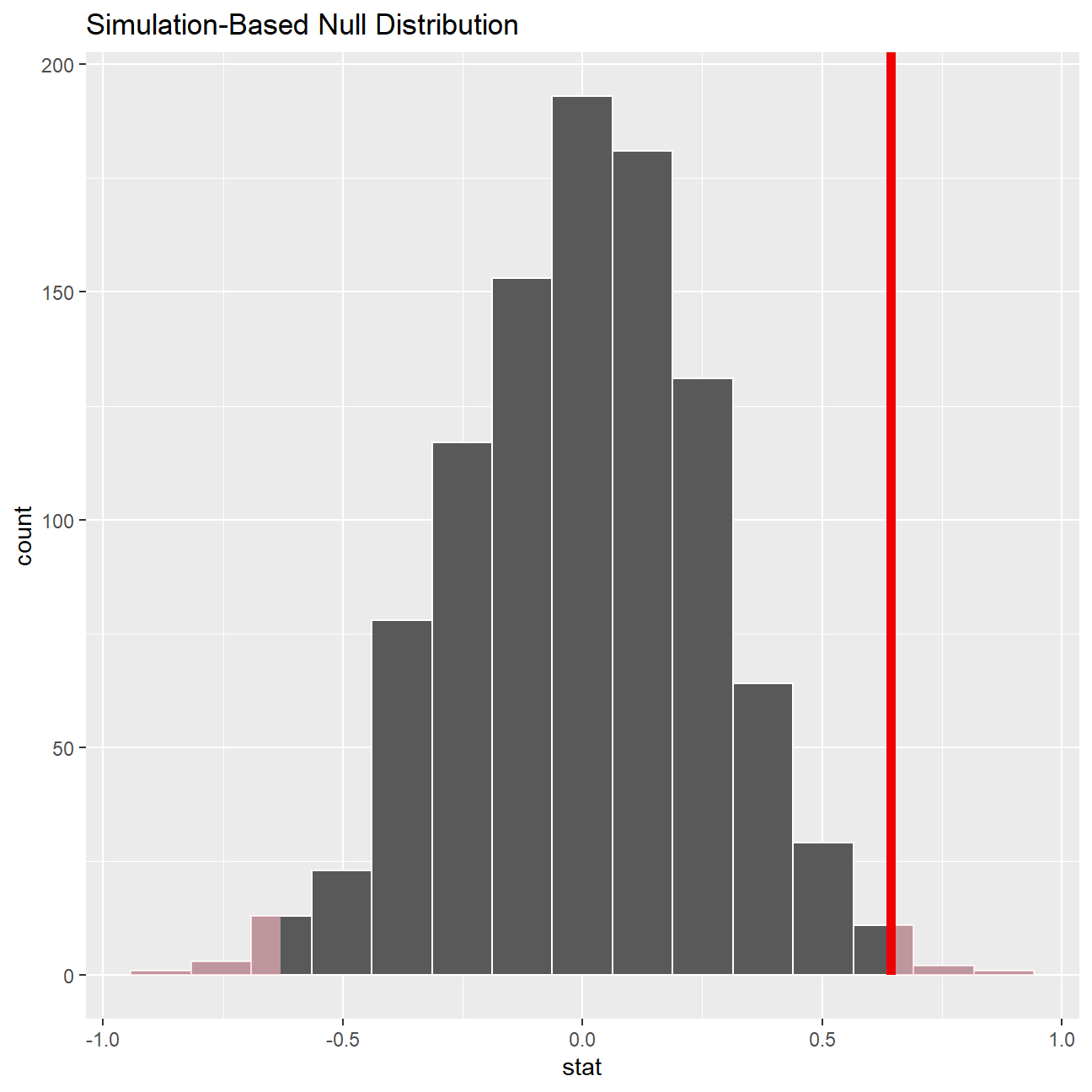
# Calculating the p-value for the hypothesis test
directors_null_dist %>%
  get_p_value(obs_stat = directors_diff, direction = "two_sided")
## # A tibble: 1 x 1
## p_value
## <dbl>
## 1 0.01From the hypothesis test, we can see that the t-stat is 3 and the p-value is 1% which is smaller than 5%, so we reject the null hypothesis and conclude that the the difference in mean IMDB ratings for Steven Spielberg and Tim Burton is statistically significant, specifically the mean rating of Steven Spielberg is higher. This is just like what we expected, as we all prefer Steven Spielberg.